ACCOUNTTURNOVER

Overview

The ACCOUNTTURNOVER function calculates the turnover of one or more general ledger account(s) as of a given period.

This is particularly useful for creating YTD, MTD, or QTD reports.

Syntax

=ACCOUNTTURNOVER(
    ConnectionName, 
    Ledger, 
    AccountClass, 
    Account, 
    Subaccount, 
    Branch, 
    FromPeriodOrDate, 
    ToPeriodOrDate, 
    IncludeUnposted, 
    UseMasterFinancialCalendar,
    UseAccountCurrency
)

Arguments

The ACCOUNTTURNOVER function uses the following arguments (see our articles on Filtering Velixo Functions and using arrays or cell ranges as arguments):

Argument	Required/Optional	Description
`ConnectionName`	Optional	Provide one of the following values: Connection name as defined in Connection Manager. Velixo range expression defining a set of connection names. An array of settings as described in the Multiple connections per formula article. We recommend using the VX.SETTINGS function to construct the array. OR Omit the argument to return results for all compatible connections with default aggregation settings.
`Ledger`	Required	Ledger ID. Leverage the ACU.EXPANDLEDGERRANGE function to obtain available values. Supports Velixo filtering techniques. When used with Budget ledgers, the `ACCOUNTTURNOVER` function returns only released budget data
`AccountClass`	Optional, though required if `Account` is empty	Account class ID. Leverage the EXPANDACCOUNTCLASSRANGE function to obtain available values. Supports Velixo filtering techniques.
`Account`	Optional, though required if `AccountClass` is empty	General ledger account code(s). Leverage the EXPANDACCOUNTRANGE function to obtain available values. Supports Velixo filtering techniques.
`Subaccount`	Optional	Subaccount code(s). Leverage the EXPANDSUBACCOUNTRANGE function to obtain available values. Supports Velixo filtering techniques.
`Branch`	Optional	Branch ID(s). Leverage the EXPANDBRANCHRANGE function to obtain available values. Supports Velixo filtering techniques.
`FromPeriodOrDate`	Required	The beginning financial period, in MM-YYYY format or a reference to a cell containing the beginning date in a valid Excel date format
`ToPeriodOrDate`	Required	The ending financial period, in MM-YYYY format. or a reference to a cell containing the ending date in a valid Excel date format
`IncludeUnposted`	Optional	1 - Include posted transactions only (default) 2 - Include Unposted transactions only 3 - Include Posted and Unposted transactions Transactions with a status of "On Hold" are excluded. When Unposted transactions are included, the following statuses are included: Balanced, Unposted, and Pending Approval. If a document is still in the AR module (e.g., Invoice), the corresponding GL batch has not yet been created, thus the balance for that document will not be reflected). The Pending Approval status is sourced from the `VelixoReportsPro-GLTranByPeriod` generic inquiry and requires the Velixo customization package version 7.1.678.24873 (20250722) or later. You can't include unposted transactions for the YTD Net Income account. If the accounts selected by your formula include it, the function returns an error stating that the balance can only be calculated for posted transactions. This applies whether you filter by financial period or by date. Excel for Windows allows the use of quotation marks around this argument. Excel for Mac and Excel Online require that it be unquoted.
`UseMasterFinancialCalendar`	Optional	Use Acumatica's Master Financial Calendar instead of the financial calendar defined within the specific tenant associated with the connection being accessed (this can be useful for consolidation reports). Possible values: `TRUE` `FALSE` (default)
`UseAccountCurrency`	Optional	Set to `TRUE` to return amounts in the account's own currency. When `FALSE`, returns amounts in the base currency. Accepted values: `TRUE`, `FALSE` Default value: `FALSE`

Examples

Given this data:

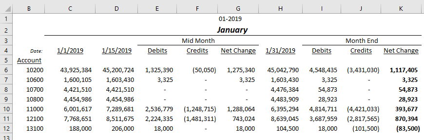
Example - Posted transactions for an account

=ACCOUNTTURNOVER(
    "Demo", 
    "ACTUAL",
    , 
    "10700", 
    , 
    , 
    "01-2019", 
    "01-2019"
)

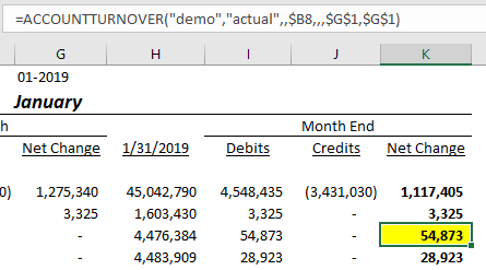
Description: Calculates the turnover of all posted transactions to General Ledger account #10700 (as noted in cell B8) during the first financial period of year 2019 (as noted in cell G1).

Result: 54,873

https://s3.ca-central-1.amazonaws.com/cdn.velixo.com/helpdesk/kIlJLxS04JN5T9eozlhJ481v7APq9Q8u2A.png

Example - Posted and Unposted transactions

=ACCOUNTTURNOVER(
    "Demo", 
    "ACTUAL",
    , 
    "10600", 
    , 
    , 
    $C$4, 
    $D$4, 
    3
)

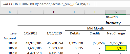
Description: Calculates the turnover of all posted and unposted transactions to General Ledger account #10600 (as noted in cell B7) between January 1, 2019 (as noted in cell C4) and January 15, 2019 (as noted in cell D4).

Result: 3,325

https://s3.ca-central-1.amazonaws.com/cdn.velixo.com/helpdesk/xYgEViSOcJAj4JukcAbVBchi-SZwsmU4fg.png

Example - Released budget values

=ACCOUNTTURNOVER(
    "Demo", 
    "BUDGET",
    , 
    "10600", 
    , 
    "*", 
    "12-2019", 
    "12-2019"
)

Description: Retrieves the released value in the Budget ledger for General Ledger account #10600 for all branches for period 12-2019

Result: 493,710

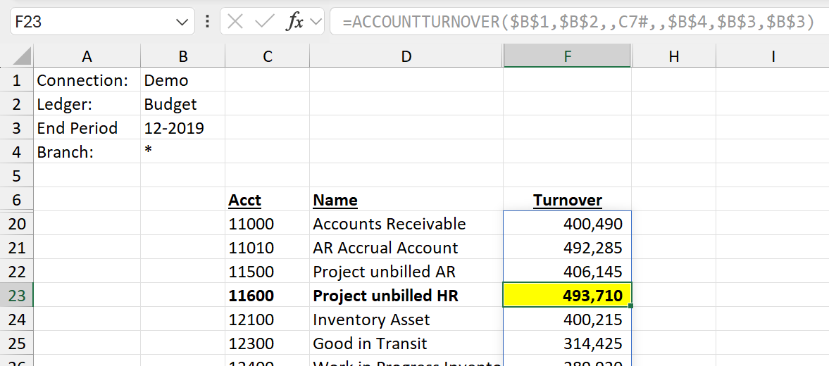
https://s3.ca-central-1.amazonaws.com/cdn.velixo.com/helpdesk/vjbrAsZe9Faw4JgKUsc4gIzR6Z42PfIIFg.png

Cell references were used for arguments in this example

Any UN-released budget values (as shown on the ERP's Release Budgets screen) will *NOT* be reflected in the balance. Only released budget values can be retrieved.

Limitations to filtering by date instead of the financial period

You can't filter the YTD Net Income account by date. This is the account set as YTD Net Income Account in Acumatica's General Ledger preferences. If the accounts selected by your formula include it, the function returns "Error! The balance of account 33000 can only be calculated by financial period since it is your net income account." Here, 33000 stands for your YTD Net Income account. To calculate net income for a date range, use the workaround below.

Drilldown will show transactions for the entire financial period (you will then need to manually filter on the date column)
Balances are calculated based on the total from the nearest financial period, and then adjusted based on the filtered transaction date
Balances will not reflect transactions within the specified date range but which have been posted to a different financial period.

Workaround: calculate net income for a date range

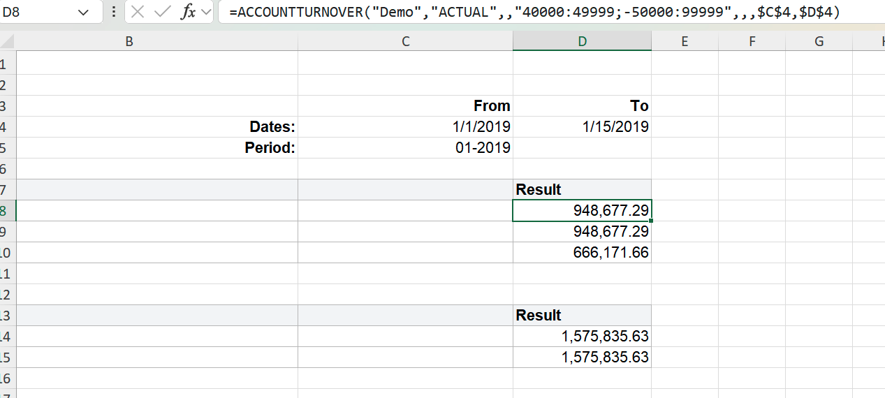
Instead of querying the YTD Net Income account, calculate net income as the total of your revenue accounts minus the total of your expense accounts. In the Account argument, enter your revenue account range, then your expense account range preceded by the subtraction operator (-). Because the two ranges don't overlap, Velixo subtracts the expense amounts from the revenue amounts. For more information, see Filtering using Velixo range expressions.

=ACCOUNTTURNOVER(
    "Demo",
    "ACTUAL",
    ,
    "40000:49999;-50000:99999",
    ,
    ,
    $C$4,
    $D$4
)

Description: Calculates net income between January 1, 2019 (cell C4) and January 15, 2019 (cell D4) as the turnover of revenue accounts 40000 to 49999 minus the turnover of expense accounts 50000 to 99999.

The account ranges come from the Demo chart of accounts. Replace them with the revenue and expense ranges from your own chart of accounts.
Make sure neither range includes your YTD Net Income account. Otherwise, the workaround doesn't give the correct result.
To check that your ranges are complete, run the formula for a full financial period and compare the result with the YTD Net Income account balance for the same period. The two values should match.
The same workaround works with ACCOUNTBEGINNINGBALANCE and ACCOUNTENDINGBALANCE. It doesn't apply to ACCOUNTTOTALDEBITS or ACCOUNTTOTALCREDITS.

If the Account balance sign option is set to Reversed, revenue amounts are returned as negative values, so subtracting expenses no longer gives net income. Instead, add both ranges without the subtraction operator, for example 40000:99999. If your ranges aren't contiguous, separate them with a semicolon, as in 40000:49999;50000:99999. For more information about this option, see Options (Classic).