What is Table Mirroring?
Many Velixo functions create Excel arrays (a single function can return multiple rows/columns).
Certain Velixo functions can express their output as either an Excel array or an Excel table, and the TOTABLE function can convert any Excel array to an Excel table.
These functions can send their entire output in unchanged order to a table (referred to as Full Mirroring mode) or can send selected columns in a specified order to the table (referred to as Per Column Mirroring mode).
To use Full Mirroring mode, use the TableOutputCell or OutputColumn1 argument of your function to define the cell address of the upper left corner of where the table is to be placed. [Leave the remaining OutputColumn# arguments (OutputColumn2, OutputColumn3, etc.) unused]
To use Per Column Mirroring mode, define all cell addresses for the columns returned by the function using OutputColumn# arguments.
Below, we explore the behavior specific to mirrored tables and provide examples of functions that use this feature.
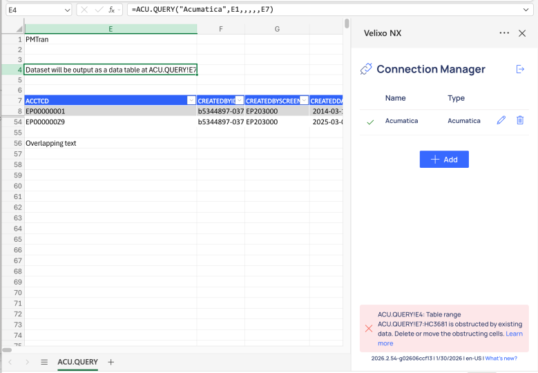
When the range of a newly created/expanded table overlaps with data already present in the worksheet, the table will not appear (new table) or will remain unchanged (updated/expanded table), and an error message will be visible in the Velixo NX side panel. Delete or move the obstructing cells to make room for the table.
Supported Velixo functions
Modifying columns in a mirrored table
You might want to modify columns in a table, or reference data which you have already used as a cell reference for another function, calculation, etc. To keep these references unaffected, a mirrored table will trigger specific Excel behavior when columns are added, removed, or their order is altered.
Adding columns
Full Mirroring mode
When a column is added, it always appears on the right side of the mirrored table, regardless of column order in the formula.
Let's look at the following formula example…
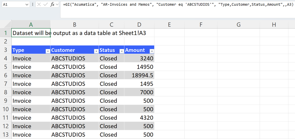
… and add a new column in the Select argument:
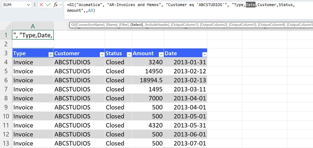
By default, the added column appears as the final column in the table, despite being the second column described in the Select argument. You can, however, modify column order at any time by dragging columns into desired positions.
Per Column Mirroring mode
This mode allows you to insert an additional column in the desired location within the mirrored table in functions that use the OutputColumn1, OutputColumn2, etc. arguments. To do so, use arguments OutputColumn1, OutputColumn2, etc. to define the order of columns.
In this formula example…
… let's add the new column as the final field in the Select argument and place it as the second column in the mirrored table:
The "Date", despite being the fifth field for the Select argument, is now the second column in the mirrored table, as the OutputColumn5 argument corresponding to this field is set to a cell address in the second column.
Removing columns
Full Mirroring mode
Remove columns as usual in Excel.
Per Column Mirroring mode
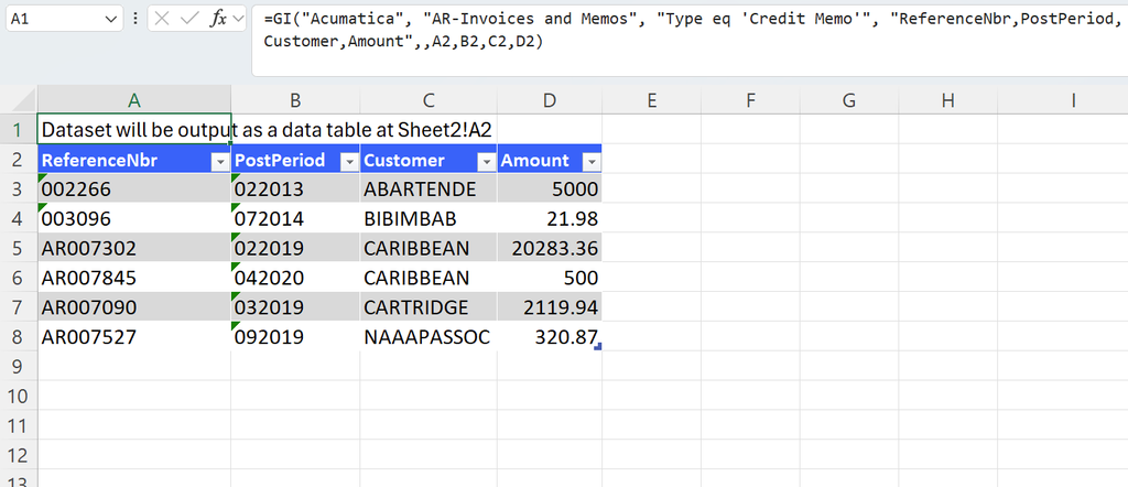
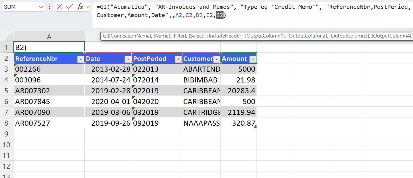
Let's remove the "PostPeriod" column from the table returned by this GI function:
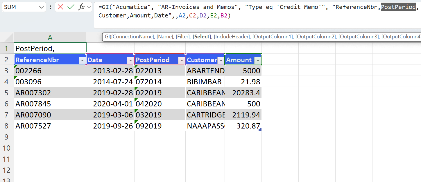
To do so, in addition to removing the "PostPeriod" field, modify the OutputColumn# arguments to take into account the number of fields in the Select argument. For instance, a scenario with four Select fields and five defined OutputColumn# arguments will result in an error.
Changing column order
Full Mirroring mode and Per Column Mirroring mode
To modify column order in a mirrored table without affecting existing references, manually drag and drop the headers in the table to achieve the desired column order:
Changing the OutputColumn# arguments will also change column order; however, doing so will break cell references to data in the rearranged columns.
Manually modifying data in a mirrored table
For data entered manually in columns added to a mirrored table to remain in their expected rows when the worksheet is refreshed, marking columns containing unique values as key columns is necessary. Data in these columns will be used to uniquely identify rows in your table.
Manually entered data will be lost once the query no longer returns key values associated with the user data.
GI function
Configure key columns by navigating to the Options menu from the Velixo NX ribbon and expanding the Generic inquiries options item. Click the edit button next to the relevant connection, click the edit button in the Key columns field, select one or more columns you would like to bind to your manually added data, and add them to the Key columns list using the down-arrow button. Confirm by clicking OK twice.
We strongly recommend selecting all columns marked with the “Key” icon, as providing key columns that are not unique can cause data to be lost.
TOTABLE function
Configure key columns by providing the column index/indexes as a field in the KeyColumnIndex argument. For instance, in this formula…
=TOTABLE(A6#, {1,2,3,4}, , I5, J5, K5, L5, M5, N5)
… the columns with indexes 1, 2, 3, and 4 become key columns.
Table mirroring in protected worksheets
If a worksheet is protected without a password, Velixo NX will automatically:
-
unprotect the worksheet just before attempting mirroring,
-
perform the mirroring operation,
-
re-protect the worksheet once the mirroring process is complete.
In the case of worksheets protected using a password, Velixo NX is not able to perform the mirroring process and will return an error.
Keeping mirroring functional in protected worksheets
The cells used to trigger mirroring, for example, dropdown cells used as filters or arguments, must remain editable and therefore cannot be “Locked”. Follow the instructions below to ensure editability.
Excel Desktop
-
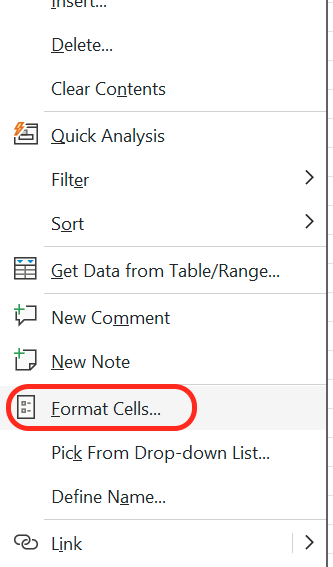
Select the relevant cells, right-click on the selection, and go to Format Cells….
-
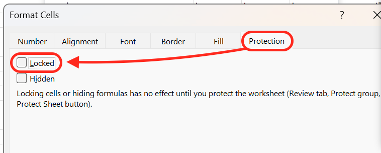
Go to the Protection tab and uncheck the Locked checkbox.
-
Protect the sheet.
Excel for the web
-
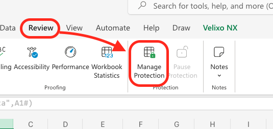
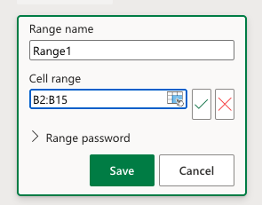
Select the relevant cells.
-
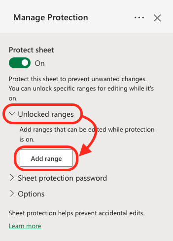
Click Manage Protection in the Protection section of the Review menu.
-
Click Add Range in the Unlocked Ranges dropdown menu.
-
Specify the parameter cells and click Save.
Function examples
TOTABLE function - convert entire array to a table (with columns in unchanged order) - Full Mirroring
=TOTABLE(B10#,,,P9)
Description
Creates a table (based on the array defined in cell B10) and places that table starting in cell P9.
Result
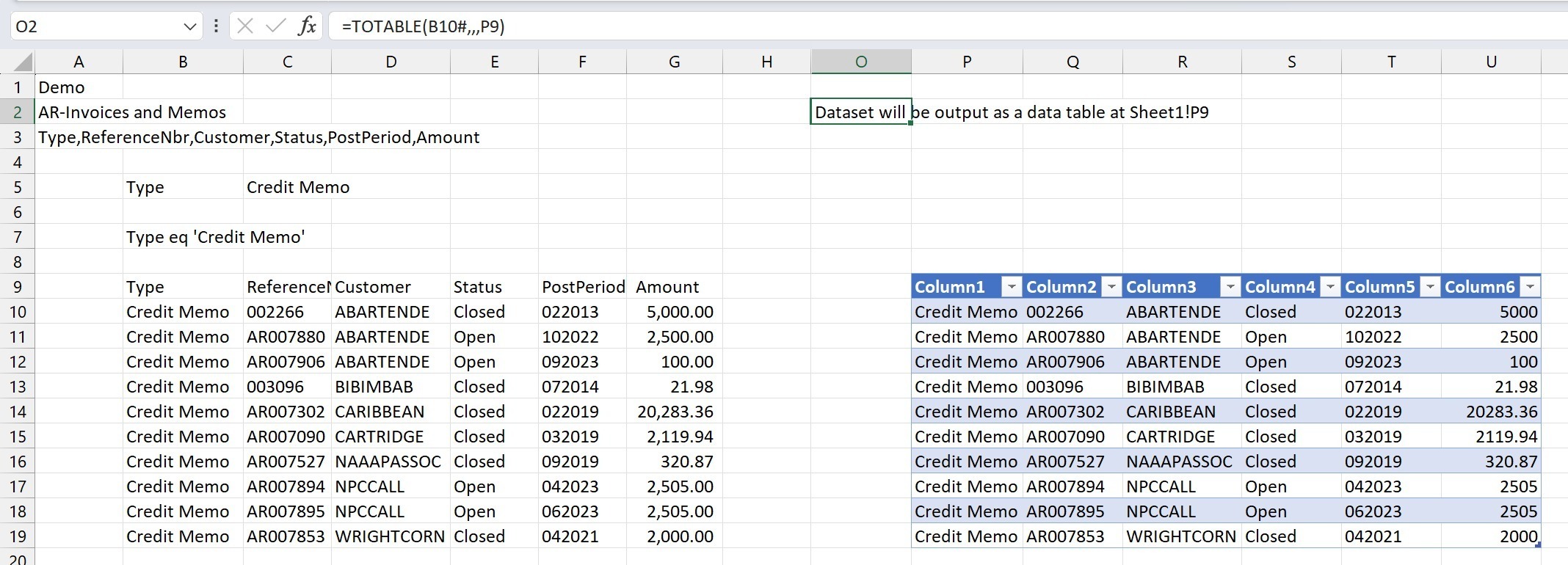
This method is referred to as Full Mirroring Mode, meaning that all the results (and ONLY the results) from the original array are included in the resulting table.
GI function - (Velixo NX only) - send entire array to a table (with columns in unchanged order) - Full Mirroring
Description
Certain Excel features do not work with Excel arrays but rather require the data to be in an Excel table. As a result, it can be convenient to have the option to create such a table from our generic inquiry data.
This example...
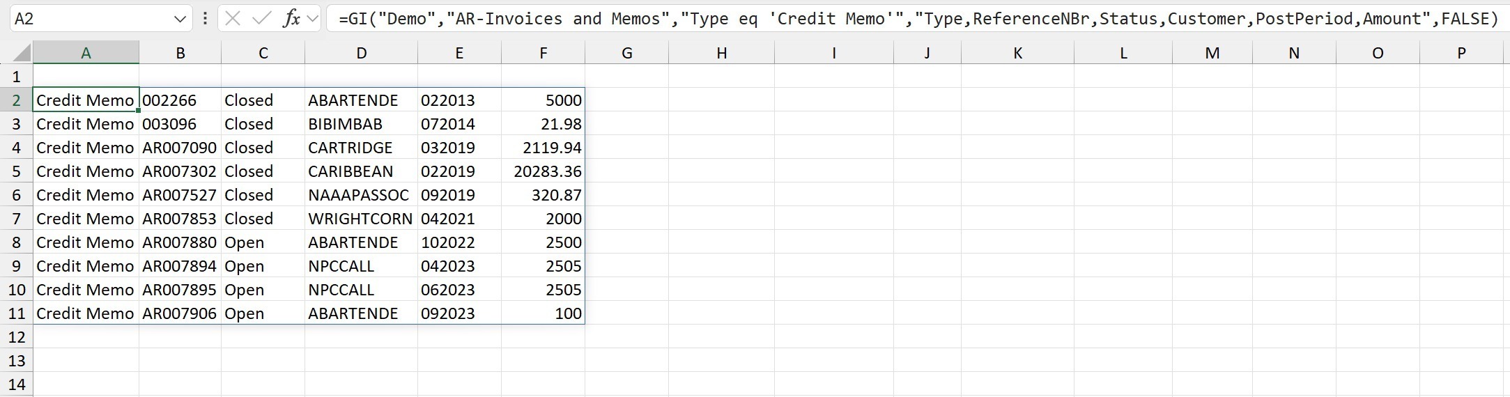
=GI("Demo", "AR-Invoices and Memos", "Type eq 'Credit Memo'", "Type,ReferenceNbr,Status,Customer,PostPeriod,Amount", FALSE)
... returns data from the AR-Invoice and Memos generic inquiry and displays it as an Excel array:
If, however, we modify the function by adding a value for the (Velixo NX only) OutputColumn1 argument...
=GI("Demo", "AR-Invoices and Memos", "Type eq 'Credit Memo'", "Type,ReferenceNbr,Status,Customer,PostPeriod,Amount", FALSE, H2)
This returns data from the generic inquiry and displays it as an Excel table starting in cell H2.
Result:
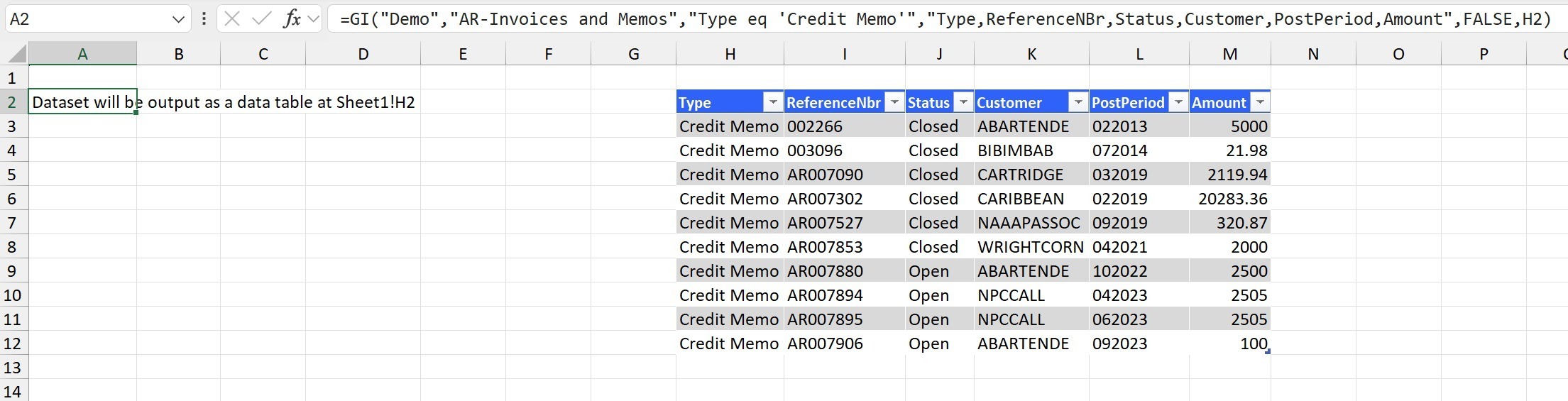
The GI() function still resides in cell A2, and the same data is returned. However, the results are displayed as an Excel table starting in the cell specified in the OutputColumn1 argument.
TOTABLE function - convert entire array to a table (changing column order) - Per-Column Mirroring
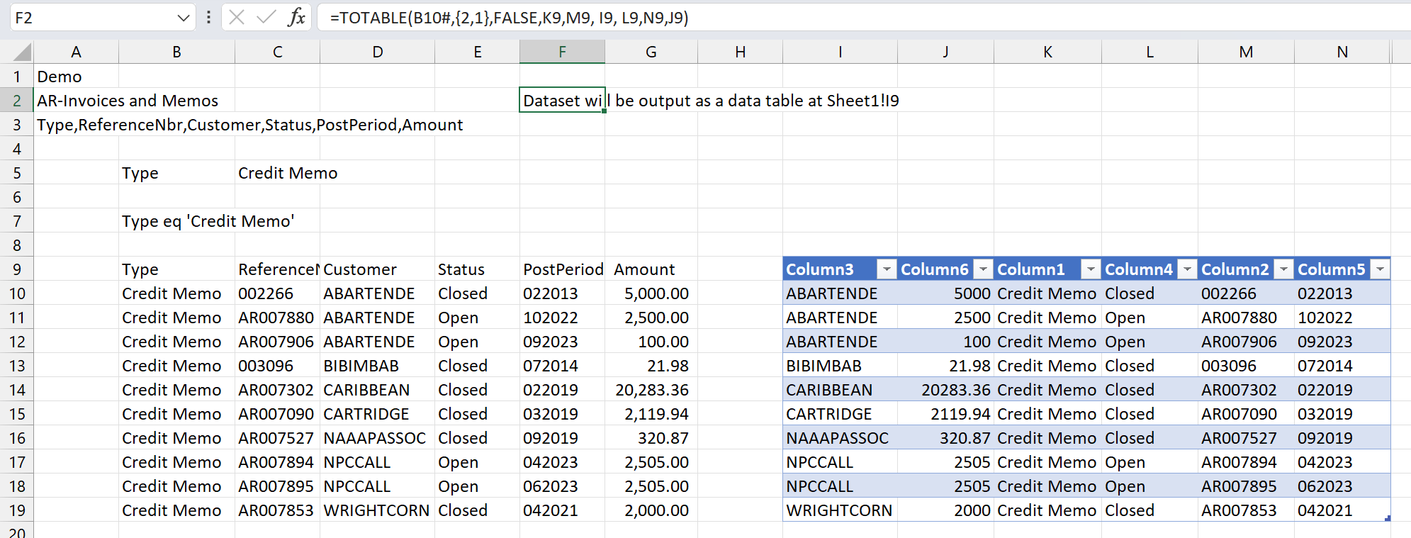
=TOTABLE(B10#, {2,1}, FALSE, K9, M9, I9, L9, N9, J9)
Description:
Creates a table (based on the results of the array defined in cell B10) as follows:
-
The second and first columns of the original array (when combined) uniquely identify each row in the array
-
The
KeyColumnIndexargument is set to:{2,1}
-
-
Header information is assumed not to be included in the array defined in cell B10
-
The
DataIncludesHeaderargument is set toFALSE
-
-
The first column of the original array will be placed in column K -
OutputColumn1is set toK9 -
The second column of the original array will be placed in column M -
OutputColumn2is set toM9 -
The third column of the original array will be placed in column I -
OutputColumn3is set toI9 -
The fourth column of the original array will be placed in column L -
OutputColumn4is set toL9 -
The fifth column of the original array will be placed in column N -
OutputColumn5is set toN9 -
The sixth column of the original array will be placed in column J -
OutputColumn6is set toJ9
This technique, where we specify both…
-
the key columns AND
-
the order for each column in the table (not just the starting cell)
... is referred to as per-column mirroring mode
Result
TOTABLE function - include (and maintain) user-entered data with the table - Per-Column Mirroring
In this example, we have added a calculation to the end of our table:
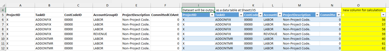
To maintain those calculated values when refreshing our report, use the per-column mirroring mode.
=TOTABLE(A5#,{1,2,3,4},TRUE,I5,J5,K5,L5,M5,N5)
Description:
This function creates a table (based on the results of the array defined in cell A5) as follows:
-
The first through fourth columns of the original array (when combined) uniquely identify each row in the array
-
The
KeyColumnIndexargument is set to:{1,2,3,4}
-
-
Header information is assumed to be included in the array defined in cell A5 (the
DataIncludesHeaderargument is set toTRUEso that the initial header row of the mirrored range is now used as a header row). -
The columns in the table will be in the same order as they appear in the original array (the specified results are to be placed in columns I through N).
By using per-column mirroring mode, when the report is refreshed, the user-specified calculations in the highlighted column will be maintained (even if the results end up displaying different records).