TOTABLE Function

Applies to:

• Velixo NX

The TOTABLE function converts an Excel array into an Excel table and places that table into the specified cell range.

TABLE OF CONTENTS

• Syntax
• Parameters
• Examples
  • Example 1 - convert entire array to table (with columns in same order) - Full Mirroring Mode
  • Example 2 - convert entire array to table (changing column order) - Per-Column Mirroring Mode
  • Example 3 - include (and maintain) user-entered data with the table - Per-Column Mirroring Mode

Syntax

TOTABLE(Array, KeyColumnIndex, DataIncludesHeader, OutputColumn1, OutputColumn2,...,OutputColumnN)

Parameters

The TOTABLE function uses the following parameters:

Examples

Example 1 - convert entire array to table (with columns in same order) - Full Mirroring Mode

=TOTABLE(B10#,,,P9)

Description

Creates a table (based on the results of the array defined in cell B10) and places that table starting in cell P9.

Result

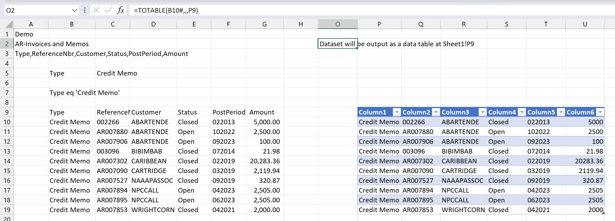
Note:  This method is referred to as Full Mirroring Mode - meaning that the entire results (and ONLY the results) from the original array are included in the resulting table.

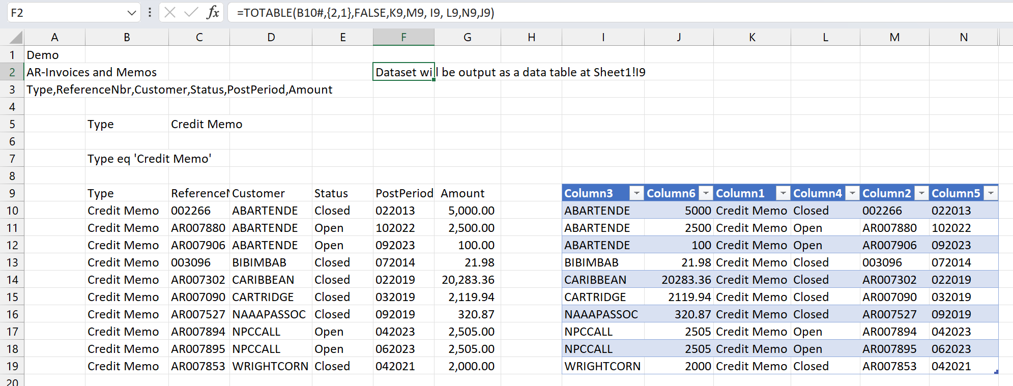
Example 2 - convert entire array to table (changing column order) - Per-Column Mirroring Mode

=TOTABLE(B10#, {2,1}, FALSE, K9, M9, I9, L9, N9, J9)

Description

Creates a table (based on the results of the array defined in cell B10) as follows:

• The second and first columns of the original array (when combined) uniquely identify each row in the array t
  • the KeyColumnIndex parameter is set to: {2,1}
• Header information is assumed to not be included in the array defined in cell B10
  • The DataIncludesHeader parameter is set to FALSE
• The first column of the original array will be placed in column K - OutputColumn1 is set to K9
• The second column of the original array will be placed in column M - OutputColumn2 is set to M9
• The third column of the original array will be placed in column I - OutputColumn3 is set to I9
• The fourth column of the original array will be placed in column L - OutputColumn4 is set to L9
• The fifth column of the original array will be placed in column N - OutputColumn5 is set to N9
• The sixth column of the original array will be placed in column J - OutputColumn6 is set to J9

This technique - where we both...

1. specify the keys columns AND 
2. specify the order for each and every column in the table (not just the starting cell)

... is referred to as per-column mirroring mode

Result

Example 3 - include (and maintain) user-entered data with the table - Per-Column Mirroring Mode

In this example, we have added a calculation to the end of our table:

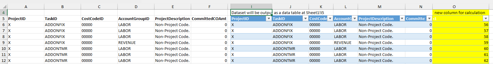
In order to maintain those calculated values when we refresh our report, we need to use per-column mirroring mode.

=TOTABLE(A6#,{1,2,3,4},,I5,J5,K5,L5,M5,N5)

Description

This function creates a table (based on the results of the array defined in cell A6) as follows:

• The first through fourth columns of the original array (when combined) uniquely identify each row in the array
  • the KeyColumnIndex parameter is set to: {1,2,3,4}
• Header information is assumed to be included in the array defined in cell A6 (the DataIncludesHeader parameter is left blank - which defaults to TRUE)
• The columns in the table will be in the same order as they appear in the original array (the specified results are to be placed in columns I through N).

By using per-column mirroring mode, when the report is refreshed, the user-specified calculations in the highlighted column will be maintained (even if the results end up displaying different records).