Applies to:

• Velixo NX
• Velixo Classic
• Every ERP

TABLE OF CONTENTS

• Overview
• Step-by-Step
  • 1 - List of Companies
  • 2 - Add a Company list to the report
  • 3 - Create a list of Company-specific Branches
  • 4 - Add a branch list pulldown to the report
  • 6 - Our report adjusts automatically

Overview

To make our reports more flexible (and avoid unnecessary changes), we try to build our reports so that they are based off a set of assumptions or parameters that we place in a centralized location.

That way, when we make a change to the parameters, our report updates automatically:

To make the example more user-friendly, would be great if the viewer did not have to remember the names of the branches but, instead, could select the desired branch from a pre-populated list.

Let's look at how we could do that.

Step-by-Step

1 - List of Companies

Let's start by assuming that our system includes a handful of companies and that each company has its own list of branches. We want to select the company and then have the list of branches update automatically.

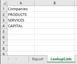
Our first step is to create a new sheet to hold our list of Companies:

2 - Add a Company list to the report

Next, we add a spot on our report where we can put the Company name:

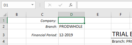
We want a pulldown list from which we can select the company we want.

After we've selected the cell where our company name will appear, we go to Excel's Data ribbon and select Data Validation. Then we tell Excel we want a List of values:

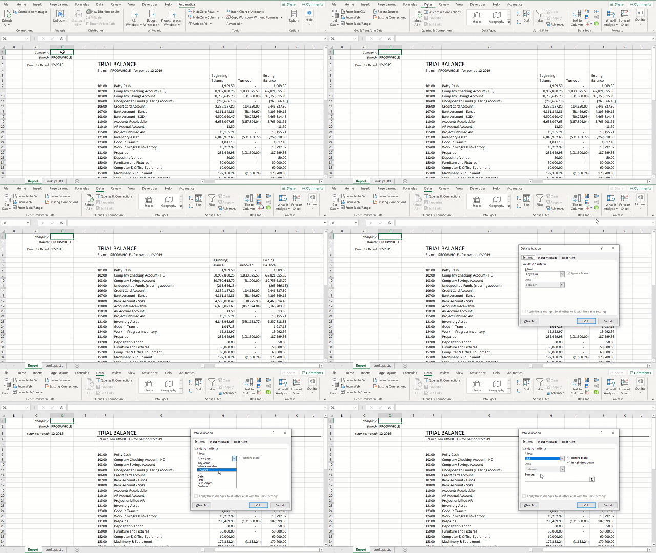
When Excel asks where to find the values we want to choose from, we select the cells containing those (and we can add extra lines to allow for future expansion):

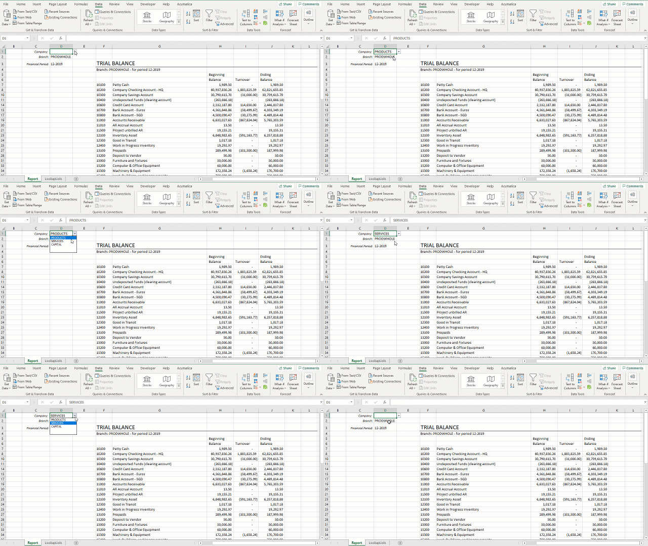
Now we can click on the arrow next to our cell, see the list of available options, and select the Company we want:

3 - Create a list of Company-specific Branches

Now we can use the Velixo BRANCHLIST function to create a list of branches for that company:

(the function references the company name in cell D1)

Once we have that list, let's make it into an Excel array by using the Velixo EXPANDBRANCHRANGE function:

4 - Add a branch list pulldown to the report

Next, let's change the branch (in our example, in cell D2) to be another pulldown list.  We'll select that cell and, just like we did for the company list, we'll use Excel's Data Validation functionality:

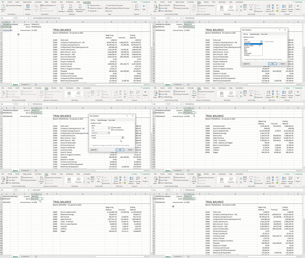
Instead of selecting a range of cells, we simply point the Source at the cell containing the list (cell A2) and then add a pound sign (#) to the end of that (=$A$1#). This allows our pulldown to grow and shrink based on the number of branches listed in column A.

6 - Our report adjusts automatically

Since our report was already configured to update (based on a change in cell B2) it continues to do so when we use the branch pulldown.